Analzying Pupil Labs Neon Data With GazeR

pupillometry

statistics

I demonstrate how to analyze pupil data from Pupil Labs Neon mobile eye-tracker with my eye-tracking R package gazeR.

Published

October 31, 2025

🎃 Happy Halloween, goils and boils! 👻

I have a spooktacular blog post for you today—one that dives into the mysterious world of pupil data from Pupil Labs Neon glasses. We’re currently using the Neon in the classroom to study mind wandering and attention. However, these mobile eye trackers aren’t just for field studies—they shine in the lab too.

To demonstrate this, I created a simple PsychoPy experiment that interfaces seamlessly with the Neon (you can find it here: https://osf.io/txz59/overview ). In the task, participants view a bright sun for 30 seconds followed by a dark patch for another 30 seconds. The pupil responds to basic visual features like brightness—constricting in light and dilating in the dark.

In this post, I’ll show how the Neon glasses can capture these pupillary dynamics and how you can use my R package {gazeR} to preprocess pupil data collected from Pupil Labs devices.

gazeR Pupil labs Functions

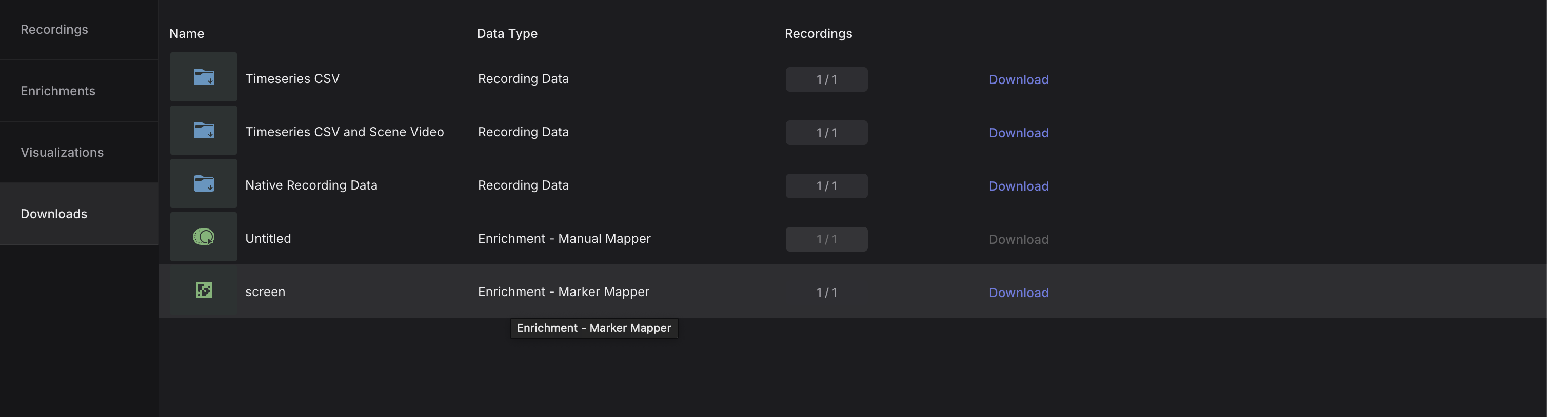
Once you collect data with Pupil Labs Neon, your recordings live in Pupil Cloud. Export the Time Series for each recording (CSV export). After the export finishes, you’ll have a folder per participant/recording containing multiple CSV files.

From each participant folder, we use exactly three files:

gaze.csv — gaze samples (timestamps, x/y pixels, fixations, blinks)

3d_eye_states.csv — pupil diameters (left/right, in mm)

events.csv — experiment events/messages (e.g., trial markers)

I created two new functions to read and process this data from Pupil Labs:

parse_pl() and process_all_subjects_PL(). Both work in tandem to prepare Neon data for use with {gazeR}.

What the functions do

parse_pl(subject_dir, aoi = FALSE, start_mode = c("any","exact"), start_messages = NULL, max_event_lag_ms = 20)

Processes one participant:

Reads the three CSVs and converts timestamps to milliseconds.
Joins pupil data to gaze samples.
Aligns each non-recording event (events.csv) to the nearest gaze row (within max_event_lag_ms).
If aoi=TRUE, it can read in the surface or AOI files. Here we used the marker mapper to map gaze on the screen of the laptop I used to record the data.
Creates trial indices:

start_mode = “any” → any non-empty message (excluding recording.begin/.end) starts a new trial.
start_mode = “exact” → only messages listed in start_messages start a new trial (robust to case/whitespace/hyphen differences).

Resets time to 0 at the first row of each trial.
Returns a tidy tibble ready for {gazeR}: subject, trial, time, x, y, pupil, blink, message.

Note

If you read in surface data, it will include whether gaze was found on the surface or not as well as x,y surface coordinates.

process_all_subjects_PL(root_dir, output_dir = file.path(root_dir, "processed"), ...)

Batch-processes all immediate subfolders of root_dir using parse_pl(), writes one CSV per subject plus a combined files

Per-subject files: {output_dir}/{SUBJECT}_processed.cs

Combined file: {output_dir}/all_subjects_processed.csv

Any additional arguments (...) are passed straight to parse_pl() (e.g., start_mode, start_messages, max_event_lag_ms).

Example Dataset

Let’s read in the dataset created from the above functions.

We will load in {gazeR} and needed libraries.

remotes::install_github("dmirman/gazer") # gazer package
library(gazer) # load in 
library(tidyverse) # viz
library(knitr) # tables

sub_pl = read.csv("https://osf.io/zf2qu/download")
kable(head(sub_pl))

subject	trial	time	x	y	pupil	blink	message
2025-10-31_12-48-26-74964918	1	0.000000	813.938	606.636	4.24975	FALSE	trial-started-light
2025-10-31_12-48-26-74964918	1	5.005127	815.400	608.674	4.21485	FALSE
2025-10-31_12-48-26-74964918	1	9.994873	815.163	607.715	4.23690	FALSE
2025-10-31_12-48-26-74964918	1	14.994629	814.249	606.579	4.25715	FALSE
2025-10-31_12-48-26-74964918	1	19.994629	812.541	607.620	4.22035	FALSE
2025-10-31_12-48-26-74964918	1	24.994873	815.149	607.083	4.20380	FALSE

Let’s take a look at the data we have.

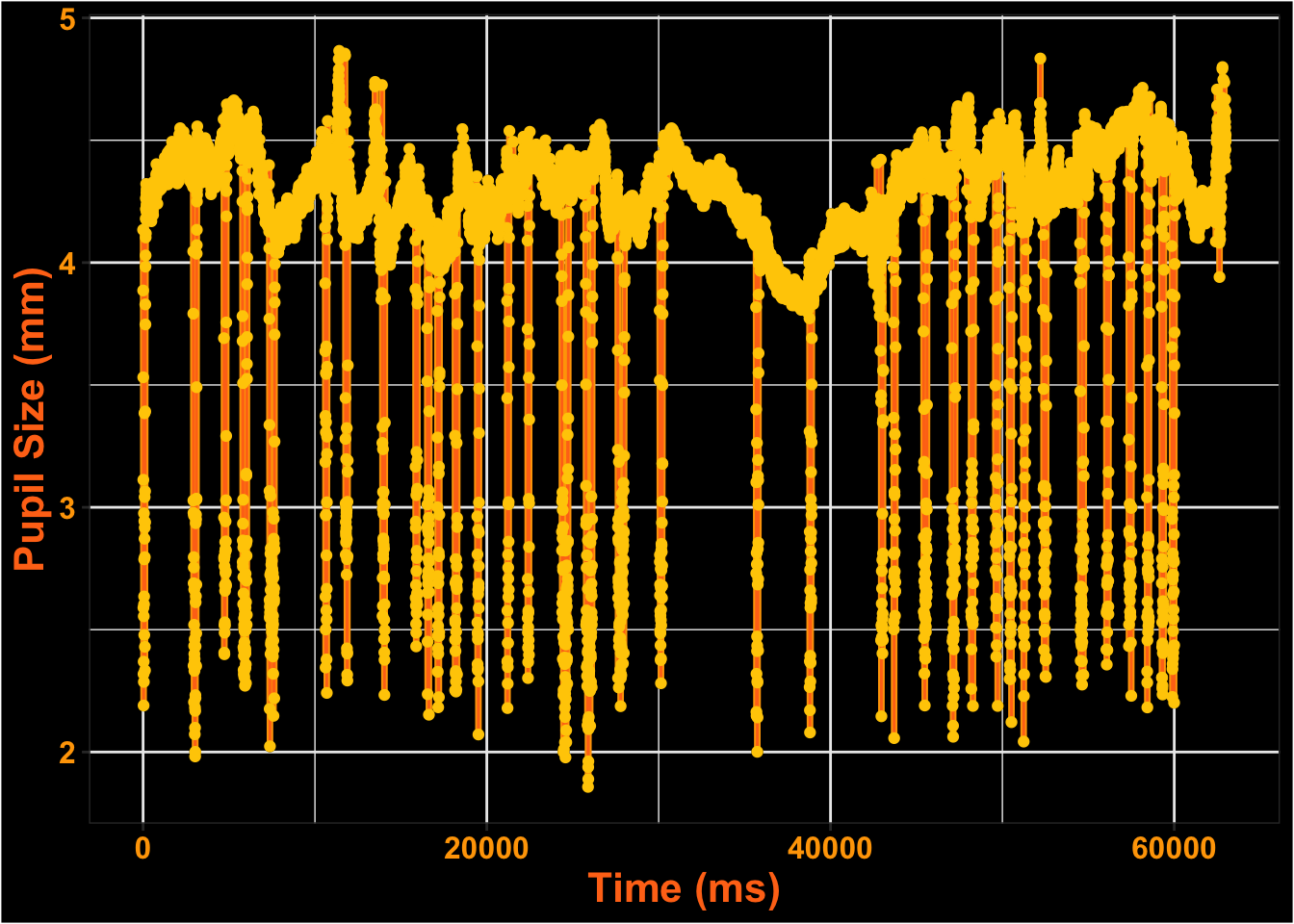
This is what the pupil data looks like for the entire time course.

Extending Blinks

We see dips in the pupil signal—these are most likely caused by blinks. Pupil Labs includes a blink detection algorithm, which we’ll use here. We first set pupil size values corresponding to blinks to NA, then use extend_blinks()to extend blinks 100 ms forward and backward in time.

  #Extend Blinks
pup_extend<- sub_pl |>
  mutate(pupil=ifelse(blink==TRUE, NA, pupil)) |>
  group_by(subject, trial) |>
  mutate(extendpupil=extend_blinks(pupil, fillback=100, fillforward=100, hz=200)) |>
  ungroup()

Interpolate blinks

Next, we linearly interpolate over blinks and smooth the data using a 5-point moving average.

# Smooth and Interpolate
smooth_interp <- smooth_interpolate_pupil(pup_extend, pupil="pupil", extendpupil="extendpupil", extendblinks=TRUE, step.first="smooth", maxgap=Inf, type="linear", hz=200, n=5)

Then, calculate missing data and remove trials with more than 50% missing data.

 pup_missing<-count_missing_pupil(smooth_interp, missingthresh = .5)

Unlikely Pupil Sizes

Now, keep only plausible pupil diameters between 2 mm and 9 mm.

pup_outliers<-pup_missing |>
  dplyr::filter (pup_interp  >= 2, pup_interp <= 9)

MAD

Get rid of artifacts we might have missed during some earlier steps.

  #MAD removal
max_removal<-pup_missing  |>
  dplyr::group_by(subject, trial) |>
  dplyr::mutate(speed=speed_pupil(pup_interp,time)) |>
  dplyr::mutate(MAD=calc_mad(speed)) |>
  dplyr::filter(speed < MAD)

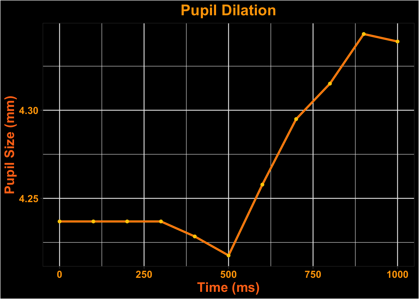
Onset

Let’s only look from the start of the trial until 1000 ms

pupil_onset<-max_removal |>
  dplyr::group_by(subject, trial) |>
  dplyr::filter(time <= 1000) |>
  select(subject, trial, time, pup_interp)

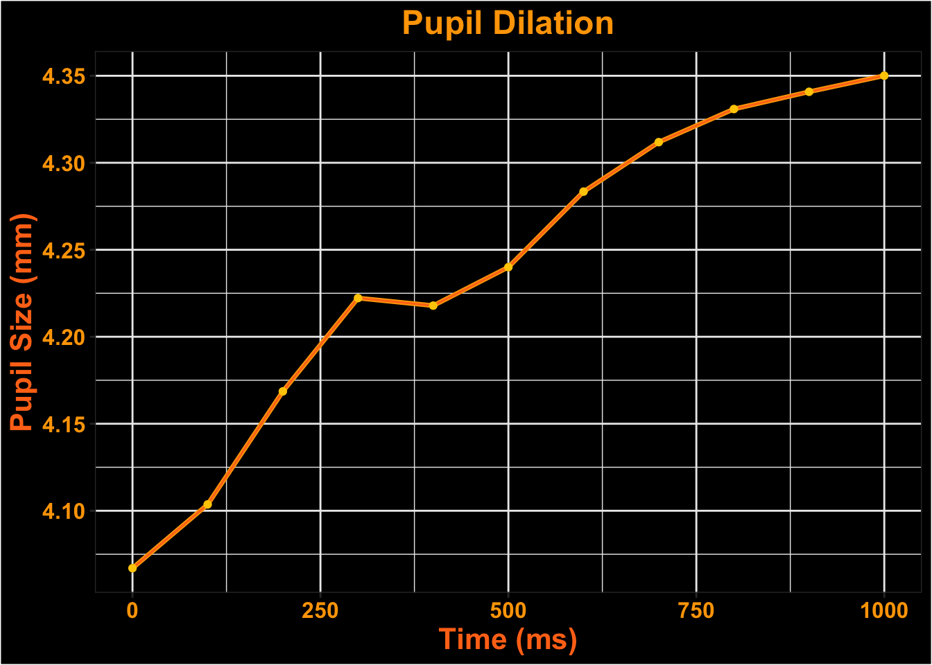
Downsample

Downsample the time-course to 100 ms.

#downsample
timebins1<- downsample_gaze(pupil_onset, bin.length=100, pupil="pup_interp", timevar = "time", aggvars = c("subject", "trial", "timebins"), type="pupil")

kable(head(timebins1))

subject	trial	timebins	aggbaseline
2025-10-31_12-48-26-74964918	1	0	4.233871
2025-10-31_12-48-26-74964918	1	100	4.251030
2025-10-31_12-48-26-74964918	1	200	4.264931
2025-10-31_12-48-26-74964918	1	300	4.296879
2025-10-31_12-48-26-74964918	1	400	4.323454
2025-10-31_12-48-26-74964918	1	500	4.247790

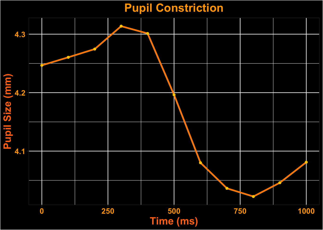
Visualize Time-course

Surface Looks

What does the data look like if we constrain the analyses to only include looks to the laptop screen?

sub_pl = read.csv("https://osf.io/enf6u/download")
kable(head(sub_pl))

subject	trial	time	gaze_detected_on_surface	gaze_position_on_surface_x_normalized	gaze_position_on_surface_y_normalized	pupil	blink	message	fixation_id
test1	1	0.000000	TRUE	0.503664	0.523080	4.28100	FALSE	trial-started-light	1
test1	1	5.000000	TRUE	0.505029	0.524774	4.24610	FALSE		1
test1	1	9.999756	TRUE	0.505353	0.521651	4.22220	FALSE		1
test1	1	15.011963	TRUE	0.505129	0.522213	4.23325	FALSE		1
test1	1	20.000000	TRUE	0.503285	0.520440	4.27000	FALSE		1
test1	1	25.000000	TRUE	0.504079	0.509780	4.25900	FALSE		1

Let’s take a look at the data we have.

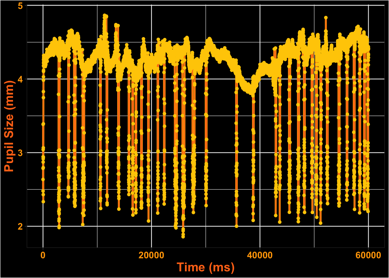
This is what the pupil data looks like for the entire time course.

Extending Blinks

  #Extend Blinks
pup_extend<- sub_pl |>
  mutate(pupil=ifelse(blink==TRUE, NA, pupil)) |>
  group_by(subject, trial) |>
  mutate(extendpupil=extend_blinks(pupil, fillback=100, fillforward=100, hz=200)) |>
  ungroup()

Interpolate blinks

Next, we linearly interpolate over blinks and smooth the data using a 5-point moving average.

# Smooth and Interpolate
smooth_interp <- smooth_interpolate_pupil(pup_extend, pupil="pupil", extendpupil="extendpupil", extendblinks=TRUE, step.first="smooth", maxgap=Inf, type="linear", hz=200, n=5)

Then, calculate missing data and remove trials with more than 50% missing data.

 pup_missing<-count_missing_pupil(smooth_interp, missingthresh = .5)

Unlikely Pupil Sizes

Now, keep only plausible pupil diameters between 2 mm and 9 mm.

pup_outliers<-pup_missing |>
  dplyr::filter (pup_interp  >= 2, pup_interp <= 9)

MAD

Get rid of artifacts we might have missed during some earlier steps.

  #MAD removal
max_removal<-pup_missing  |>
  dplyr::group_by(subject, trial) |>
  dplyr::mutate(speed=speed_pupil(pup_interp,time)) |>
  dplyr::mutate(MAD=calc_mad(speed)) |>
  dplyr::filter(speed < MAD)

Onset

Let’s only look from the start of the trial until 1000 ms

pupil_onset<-max_removal |>
  dplyr::group_by(subject, trial) |>
  dplyr::filter(time <= 1000, gaze_detected_on_surface==TRUE) |>
  select(subject, trial, time, pup_interp)

Downsample

Downsample the time-course to 100 ms.

#downsample
timebins1<- downsample_gaze(pupil_onset, bin.length=100, pupil="pup_interp", timevar = "time", aggvars = c("subject", "trial", "timebins"), type="pupil")

kable(head(timebins1))

subject	trial	timebins	aggbaseline
test1	1	0	4.246710
test1	1	100	4.260450
test1	1	200	4.274502
test1	1	300	4.313692
test1	1	400	4.301169
test1	1	500	4.196293

Visualize Time-course